33  (WIP) Boundary Problems - Refining Solutions

33.1 Evolving a solution

The sheer number of possible solutions makes this a tricky problem to solve!

We could keep generating a very large number of random solutions, and this may work to eventually find a near-optimal solution, but could be extremely time-consuming and resource-intensive, requiring many hours of compute power.

Instead, let’s try taking some inspiration from the natural world and evolving our solutions until they are as good as can be.

Tip

This is a big part of the field of operational research, with certain algorithms like NSGA-II being well-known and defined, and implemented in libraries that you can reuse. However, you can also create your own genetic algorithms or modify approaches like NSGA-II, as done in Allen et al. and their work on hyperacute stroke unit modelling.

Note

Due to the requirements for solutions to follow certain rules, evolving our solutions is somewhat more complex than in the case of our location allocation problem, where any combination of centres was theoretically ‘valid’. In that instance, we could randomly permute or mix solutions with no concerns surrounding what the output looked like beyond not being an exact duplicate of an already-evaluated solution. Here, with a need to generate a solution that conforms to rules like the dispatcher’s patch being continuous and all regions being allocated to one (and only one) dispatcher.

So what will the process look like in this case?

• We will generate a new random solution using our function from the previous section
• We will evaluate that solution
  • While we will initially be evaluating this solution against a single metric, the same approach could be applied when scoring against multiple metrics
• If this solution is worse than the current status quo, we will generate a new random solution (and keep doing so until we find a solution that performs ‘better’ than the current status quo)
• If this solution is better than the current status quo, we will then start to evolve this solution
  • for each ‘player’ (in this case, our dispatchers), we will randomly add or remove a small number of their regions and allocate it to one of the other players for whom it would be valid territory (i.e. they share a boundary with the territory in question)
    • we will generate many of these variants per round
    • we will then assess the performance of each of these solutions
    • several of the best solutions (a parameter we will be able to vary) will be retained at this point, going on to form a new population of solutions we can continue to loop through, tweak, and recheck the performance of
      • rather than the ‘child’ solutions replacing the ‘parents’, we will keep both at each stage, evaluating them all on their merits rather than always assuming the ‘child’ strategies will be better
      • note that general recommendations are that 𝝺 - the population size - should be at least 10 times larger than μ - the number of solutions we keep in each generation
      • it’s also recommended that 𝝺 / μ should leave no remainder
  • we will continue this process until there has been no improvement for several rounds of attempts
    • the number of rounds for which there is no improvement will be a parameter we can vary
• We will then store the performance of this solution, then start with a new random solution and repeat this for a certain number of solutions or period of time

Tip

As the minor variation and evaluation of solutions is much quicker than generating brand new solutions with the method we developed in the previous chapter, we should see much faster movement towards a ‘good’ solution. This approach should therefore be more efficient than if we were to use the same amount of computational time generating and evaluating random solutions (though there is a small chance we land on a great solution at random!).

However, it should also be remembered that there is something to be said for a simple approach…

“Experience shows that if the stakeholders (users of the model) can easily understand the methods used, they are more likely to trust the solution and use the model more confidently in the decision making processes” - Meskarian R, Penn ML, Williams S, Monks T (2017)¹

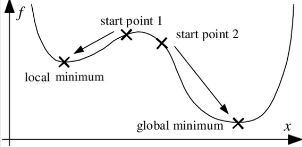
33.2 Local and Global Optima

²

Evolutionary algorithms can have the issue of getting stuck in local optima - where they reach a ‘good’ solution and small tweaks in any direction lead to worse scores. However, outside of the ‘sight’ of the algorithm, there may be a better overall solution that exists.

While there are a range of ways this issue can be tackled, here we’ll mainly be approaching it by working with several different random starting positions.

33.3 Loading Previous Solutions

To start with, let’s load our random solutions from the last chapter back in.

Warning

Pickle is a convenient file format for storing dataframes and reloading them with important information like column types retained. This is important in situations like this where one of our columns is a more complex datatype that may not transfer well into a csv.

However, pickle is not particularly secure and you should only unpickle files from sources you trust as there is a risk of malicious code being injected and then executing on unpickling. Alternative formats such as Feather and Parquet are generally regarded as more secure.

import pandas as pd

initial_solution_df = pd.read_pickle('solutions_example.pkl')

initial_solution_df.to_csv('solutions_example.csv')

Let’s write a quick function to pull out the allocations from our solutions file, and turn that back into a dataframe we can work with.

def extract_allocation_df_from_solution_df(df, solution_rank, allocation_col_name, territory_col_name):
    row_of_interest = df[df['rank'] == solution_rank]
    owned_territory_dict = row_of_interest['allocations'].values[0]

    owned_territory_df = pd.DataFrame(
            [(key, value) for key, values in owned_territory_dict.items() for value in values],
            columns=[allocation_col_name, territory_col_name])
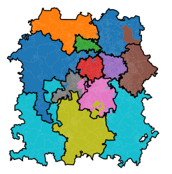
    return owned_territory_df

Let’s now try this out to pull back and visualise our best solution.

best_solution = extract_allocation_df_from_solution_df(
    initial_solution_df,
    solution_rank=1,
    allocation_col_name="centre_dispatcher_NEW",
    territory_col_name="LSOA11CD"
    )

best_solution

	centre_dispatcher_NEW	LSOA11CD
0	Centre 2-5	E01031187
1	Centre 2-5	E01031195
2	Centre 2-5	E01031217
3	Centre 2-5	E01031204
4	Centre 2-5	E01031213
...	...	...
2006	Centre 2-2	E01009724
2007	Centre 2-2	E01009720
2008	Centre 2-2	E01009723
2009	Centre 2-2	E01009725
2010	Centre 2-2	E01009730

2011 rows × 2 columns

Click here to view code from previous chapters for importing our historical boundary and demand data

import geopandas

lsoa_geojson_path = 'https://github.com/hsma-programme/h6_3c_interactive_plots_travel/raw/main/h6_3c_interactive_plots_travel/example_code/LSOA_2011_Boundaries_Super_Generalised_Clipped_BSC_EW_V4.geojson'

lsoa_boundaries = geopandas.read_file(lsoa_geojson_path)

xmin, xmax = 370000, 420000
ymin, ymax = 250000, 310000

bham_region = lsoa_boundaries.cx[xmin:xmax, ymin:ymax]

bham_region["region"] = bham_region["LSOA11NM"].str[:-5]

boundary_allocations_df = pd.read_csv("boundary_allocations.csv")

bham_region = pd.merge(
    bham_region,
    boundary_allocations_df,
    left_on="region",
    right_on="Region",
    how="left"
)

bham_region["centre_dispatcher"] = bham_region["Centre"].astype("str") + '-' + bham_region["Dispatcher"].astype("str")

demand = pd.read_csv("demand_pop_bham.csv")

bham_region = bham_region.merge(demand, on="LSOA11CD")

# Create df of original boundaries
grouped_dispatcher_gdf = bham_region.groupby("centre_dispatcher")

# Create a new GeoDataFrame for the boundaries of each group
boundary_list = []

for group_name, group in grouped_dispatcher_gdf:
    # Combine the polygons in each group into one geometry
    combined_geometry = group.unary_union

    # Get the boundary of the combined geometry
    boundary = combined_geometry.boundary

    # Add the boundary geometry and the group name to the list
    boundary_list.append({'group': group_name, 'boundary': boundary})

# Create a GeoDataFrame from the list of boundaries
grouped_dispatcher_gdf_boundary = geopandas.GeoDataFrame(boundary_list, geometry='boundary', crs=bham_region.crs)

/home/sammi/.local/lib/python3.10/site-packages/geopandas/geodataframe.py:1528: SettingWithCopyWarning:


A value is trying to be set on a copy of a slice from a DataFrame.
Try using .loc[row_indexer,col_indexer] = value instead

See the caveats in the documentation: https://pandas.pydata.org/pandas-docs/stable/user_guide/indexing.html#returning-a-view-versus-a-copy

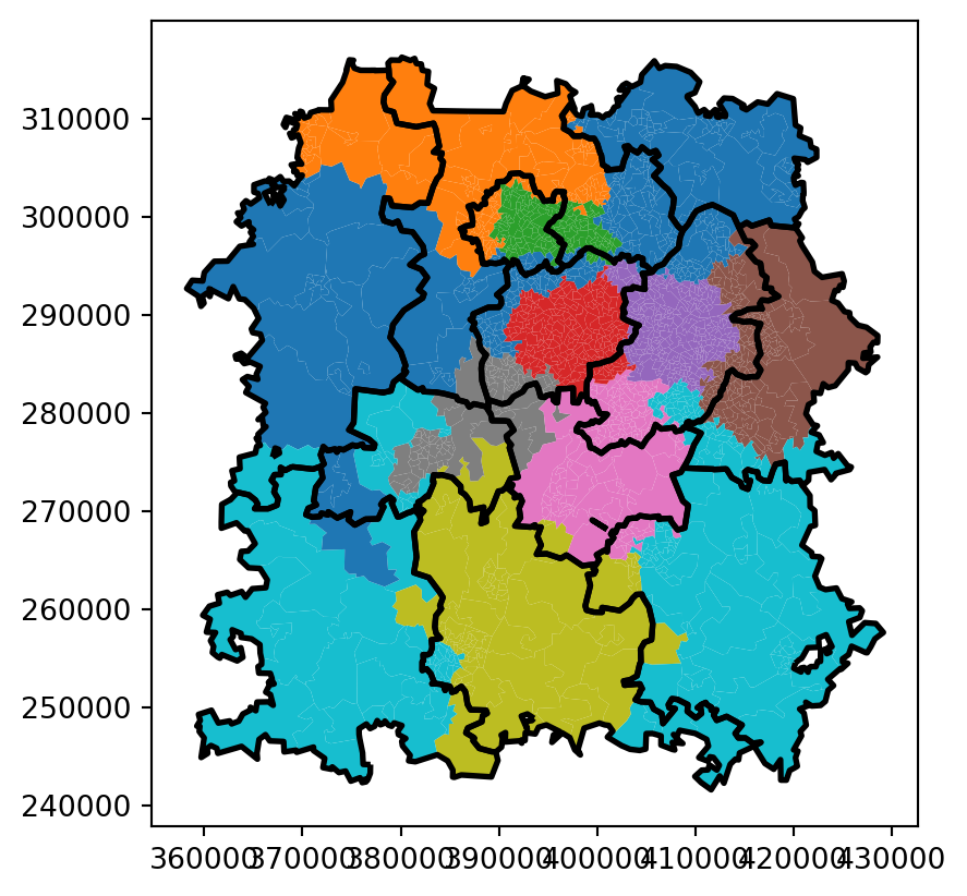
ax=bham_region.merge(best_solution, on="LSOA11CD").plot(column="centre_dispatcher_NEW")

# Visualise the historical boundaries
grouped_dispatcher_gdf_boundary.plot(
    ax=ax,
    linewidth=2,
    edgecolor="black"
)

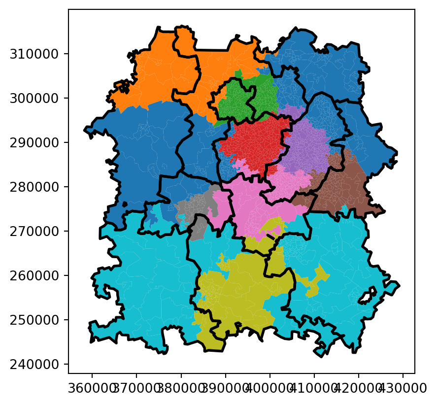
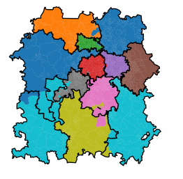
And let’s compare this with our worst-performing solution.

Click here to see the code

worst_solution = extract_allocation_df_from_solution_df(
    initial_solution_df,
    solution_rank=20,
    allocation_col_name="centre_dispatcher_NEW",
    territory_col_name="LSOA11CD"
    )

ax=bham_region.merge(worst_solution, on="LSOA11CD").plot(column="centre_dispatcher_NEW")

# Visualise the historical boundaries
grouped_dispatcher_gdf_boundary.plot(
    ax=ax,
    linewidth=2,
    edgecolor="black"
)

33.4 Writing our evolutionary algorithm

Click here for a reminder of what we are trying to code in our evolutionary algorithm

• If this solution is better than the current status quo, we will then start to evolve this solution
  • for each ‘player’ (in this case, our dispatchers), we will randomly add or remove a small number of their regions and allocate it to one of the other players for whom it would be valid territory (i.e. they share a boundary with the territory in question)
    • we will generate many of these variants per round
    • we will then assess the performance of each of these solutions
    • several of the best solutions (a parameter we will be able to vary) will be retained at this point, going on to form a new population of solutions we can continue to loop through, tweak, and recheck the performance of
      • rather than the ‘child’ solutions replacing the ‘parents’, we will keep both at each stage, evaluating them all on their merits rather than always assuming the ‘child’ strategies will be better
      • note that general recommendations are that 𝝺 - the population size - should be at least 10 times larger than μ - the number of solutions we keep in each generation
      • it’s also recommended that 𝝺 / μ should leave no remainder
  • we will continue this process until there has been no improvement for several rounds of attempts
    • the number of rounds for which there is no improvement will be a parameter we can vary
• We will then store the performance of this solution, then start with a new random solution and repeat this for a certain number of solutions or period of time

We’re also going to reuse our ‘add_neighbours_column()’ function from before.

Click here to view the add_neighbours_column() function from the previous chapter

def add_neighbors_column(gdf):
    """
    Adds a column to the GeoDataFrame containing lists of indices of neighboring polygons
    based on the 'touches' method.
    """
    gdf = gdf.copy()
    neighbors = []
    for idx, geom in gdf.geometry.items():
        touching = gdf[gdf.geometry.touches(geom)]["LSOA11CD"].tolist()
        neighbors.append(touching)

    gdf["neighbors"] = neighbors
    return gdf

def find_border_dispatchers(row, df, allocation_colname='centre_dispatcher_NEW'):
    current_dispatcher = row[allocation_colname]
    neighbors = row['neighbors']

    # Get dispatchers of neighboring LSOAs
    neighboring_dispatchers = {
        df.loc[df['LSOA11CD'] == neighbor, allocation_colname].values[0]
        for neighbor in neighbors if not df[df['LSOA11CD'] == neighbor].empty
    }

    # Filter to only different dispatchers
    border_dispatchers = list(neighboring_dispatchers - {current_dispatcher})

    return border_dispatchers if border_dispatchers else []

import random
import networkx as nx
from shapely.geometry import MultiPolygon
from shapely.ops import unary_union

def is_solution_continuous(solution_gdf, allocation_col):
    """
    Checks if all dispatcher-assigned regions are contiguous.
    """

    # Dissolve regions by dispatcher
    dispatcher_groups = solution_gdf.dissolve(by=allocation_col)

    for geom in dispatcher_groups.geometry:
        # If the region is a single Polygon, it's already contiguous
        if not isinstance(geom, MultiPolygon):
            continue  # No need to check further

        # Build a connectivity graph
        G = nx.Graph()
        parts = list(geom.geoms)  # Extract individual polygons

        # Add polygons as nodes
        for i in range(len(parts)):
            G.add_node(i)

        # Connect nodes if polygons overlap or touch
        for i in range(len(parts)):
            for j in range(i + 1, len(parts)):
                if parts[i].intersects(parts[j]):  # Stronger than .touches()
                    G.add_edge(i, j)

        # Check if all polygons form one connected component
        if nx.number_connected_components(G) > 1:
            return False  # Found disconnected parts

    return True

def is_continuous_after_swap(solution_gdf, lsoa,
                             current_dispatcher,
                             proposed_dispatcher,
                             allocation_col):
    """
    Checks if assigning 'lsoa' to 'new_dispatcher' maintains contiguous regions.
    This version avoids making a full DataFrame copy.
    """
    # Temporarily assign new dispatcher
    solution_gdf.loc[solution_gdf["LSOA11CD"] == lsoa, allocation_col] = proposed_dispatcher

    # Check continuity
    is_valid = is_solution_continuous(solution_gdf, allocation_col)

    # Revert change immediately (avoiding full copy overhead)
    solution_gdf.loc[solution_gdf["LSOA11CD"] == lsoa, allocation_col] = current_dispatcher

    return is_valid
    #return True

def assign_new_dispatcher(row,
                          solution_gdf,
                          border_colname,
                          permutation_chance_per_border,
                          new_allocation_colname
                          ):
        """
        Attempts to assign a new dispatcher while keeping the solution continuous.
        """

        # If no bordering dispatchers, keep the original
        if not row[border_colname]:
            #print(f'No borders in {row["LSOA11CD"]}')
            return row[new_allocation_colname]

        # If some bordering dispatchers, then randomly sample whether we will try to permute it
        elif random.uniform(0.0, 1.0) < permutation_chance_per_border:

            # Randomly select from border dispatchers
            current_dispatcher = row[new_allocation_colname]
            random_dispatcher = random.choice(row[border_colname])

            # Check if assigning this dispatcher keeps the solution contiguous
            if is_continuous_after_swap(solution_gdf,
                                        lsoa = row["LSOA11CD"],
                                        current_dispatcher=current_dispatcher,
                                        proposed_dispatcher=random_dispatcher,
                                        allocation_col=new_allocation_colname):
                #print(f"*** Swapped {row['LSOA11CD']} to {random_dispatcher} ***")
                return random_dispatcher
            else:
                #print(f":( Tried{row['LSOA11CD']} from {current_dispatcher} to {random_dispatcher}")
                return row[new_allocation_colname]  # Default to original allocation
        else:
            #print(f"Not trying to permute {row['LSOA11CD']}")
            return row[new_allocation_colname]

from joblib import Parallel, delayed

def create_evolved_solutions(
        initial_solution_df, geodataframe,
        join_col_left, join_col_right,
        original_allocation_colname='centre_dispatcher',
        random_solution_allocation_colname='centre_dispatcher_NEW',
        new_allocation_colname='centre_dispatcher_evolved',
        border_colname='border_dispatchers',
        permutation_chance_per_border=0.2,
        population_size=1
    ):
    """
    Generates evolved dispatcher allocations while ensuring that all regions remain contiguous.
    """

    # Merge initial solution with geodataframe to keep it as a geodataframe
    initial_solution_gdf = geodataframe.merge(initial_solution_df, left_on=join_col_left, right_on=join_col_right)

    # Compute neighbors and border dispatchers
    initial_solution_gdf = add_neighbors_column(initial_solution_gdf)
    initial_solution_gdf[border_colname] = initial_solution_gdf.apply(
        find_border_dispatchers, axis=1, df=initial_solution_gdf
        )

    # new_allocation_dfs = []

    # Include new_allocation_colname from the start
    simplified_allocation_df = (
        initial_solution_gdf[
            [random_solution_allocation_colname, 'LSOA11CD', border_colname, "geometry"]
            ].copy()
            )

    simplified_allocation_df[new_allocation_colname] = (
        simplified_allocation_df[random_solution_allocation_colname]
        )

    def process_iteration(i, simplified_allocation_df, border_colname,
                     permutation_chance_per_border, new_allocation_colname):

        # for i in range(population_size):
        evolved_df = simplified_allocation_df.copy(deep=True)

        # Separate out the cols with and without borders
        non_borders_df = evolved_df[evolved_df[border_colname].apply(len) == 0]
        borders_df = evolved_df[evolved_df[border_colname].apply(len) > 0]
        print(f"{len(non_borders_df)} regions without borders and {len(borders_df)} with borders")

        borders_df[new_allocation_colname] = borders_df.apply(
            lambda row: assign_new_dispatcher(
                row, borders_df,
                border_colname,
                permutation_chance_per_border,
                new_allocation_colname
                ), axis=1)

        return pd.concat([non_borders_df, borders_df], ignore_index=True)

        # evolved_df = pd.concat([non_borders_df, borders_df], ignore_index=True)

        #new_allocation_dfs.append(evolved_df.copy(deep=True))

        del evolved_df, non_borders_df, borders_df

    return Parallel(n_jobs=-1, verbose=10)(
            delayed(process_iteration)(
                i,
                simplified_allocation_df,
                border_colname,
                permutation_chance_per_border,
                new_allocation_colname
            )
            for i in range(population_size)
        )

solution = create_evolved_solutions(
    best_solution,
    bham_region,
    join_col_left="LSOA11CD",
    join_col_right="LSOA11CD",
    population_size=1
)

solution[0]

	centre_dispatcher_NEW	LSOA11CD	border_dispatchers	geometry	centre_dispatcher_evolved
0	Centre 1-7	E01008888	[]	POLYGON ((413420.692 284795.501, 413826.348 28...	Centre 1-7
1	Centre 1-7	E01008891	[]	POLYGON ((413031.049 284196.638, 413321.825 28...	Centre 1-7
2	Centre 1-7	E01008893	[]	POLYGON ((412949.766 283625.900, 412594.358 28...	Centre 1-7
3	Centre 1-7	E01008895	[]	POLYGON ((413166.349 283295.822, 413132.000 28...	Centre 1-7
4	Centre 1-6	E01008896	[]	POLYGON ((412405.000 286300.615, 412535.675 28...	Centre 1-6
...	...	...	...	...	...
2006	Centre 1-6	E01033562	[Centre 2-1, Centre 1-5]	POLYGON ((404432.818 284070.885, 404516.073 28...	Centre 1-6
2007	Centre 1-6	E01033631	[Centre 2-1]	POLYGON ((405950.078 285312.998, 405575.210 28...	Centre 2-1
2008	Centre 2-1	E01033634	[Centre 1-6]	POLYGON ((404873.774 282636.291, 404623.886 28...	Centre 2-1
2009	Centre 1-6	E01033641	[Centre 1-7]	POLYGON ((410005.374 283902.287, 410505.181 28...	Centre 1-6
2010	Centre 1-6	E01033648	[Centre 2-5]	POLYGON ((408199.966 283979.204, 408378.884 28...	Centre 2-5

2011 rows × 5 columns

33.4.1 Confirming solutions are valid

Let’s now visualise this.

We will first create a df showing the boundaries of our plots in our original solution.

# Create df of original boundaries
grouped_dispatcher_gdf_starting_solution = bham_region.merge(best_solution, on="LSOA11CD").groupby("centre_dispatcher_NEW")

# Create a new GeoDataFrame for the boundaries of each group
boundary_list = []

for group_name, group in grouped_dispatcher_gdf_starting_solution:
    # Combine the polygons in each group into one geometry
    combined_geometry = group.unary_union

    # Get the boundary of the combined geometry
    boundary = combined_geometry.boundary

    # Add the boundary geometry and the group name to the list
    boundary_list.append({'group': group_name, 'boundary': boundary})

# Create a GeoDataFrame from the list of boundaries
grouped_dispatcher_gdf_starting_solution = geopandas.GeoDataFrame(boundary_list, geometry='boundary', crs=bham_region.crs)

Then we can plot the solution, comparing it with the boundaries prior to evolution.

ax = solution[0].plot(column="centre_dispatcher_evolved", legend=True,
                      legend_kwds={'bbox_to_anchor': (1.4, 1)})

# Plot historical boundaries
grouped_dispatcher_gdf_starting_solution.plot(ax=ax, linewidth=1, edgecolor="black")

ax.axis("off")  # Hide axes for better visualization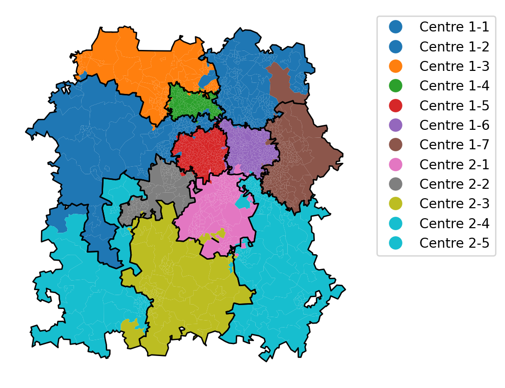

33.4.2 Generating multiple solutions at once

Let’s try generating more.

We now see benefits to having a solution with multiple outputs.

solution = create_evolved_solutions(
    best_solution,
    bham_region,
    join_col_left="LSOA11CD",
    join_col_right="LSOA11CD",
    population_size=30
)

solution[25]

	centre_dispatcher_NEW	LSOA11CD	border_dispatchers	geometry	centre_dispatcher_evolved
0	Centre 1-7	E01008888	[]	POLYGON ((413420.692 284795.501, 413826.348 28...	Centre 1-7
1	Centre 1-7	E01008891	[]	POLYGON ((413031.049 284196.638, 413321.825 28...	Centre 1-7
2	Centre 1-7	E01008893	[]	POLYGON ((412949.766 283625.900, 412594.358 28...	Centre 1-7
3	Centre 1-7	E01008895	[]	POLYGON ((413166.349 283295.822, 413132.000 28...	Centre 1-7
4	Centre 1-6	E01008896	[]	POLYGON ((412405.000 286300.615, 412535.675 28...	Centre 1-6
...	...	...	...	...	...
2006	Centre 1-6	E01033562	[Centre 2-1, Centre 1-5]	POLYGON ((404432.818 284070.885, 404516.073 28...	Centre 1-6
2007	Centre 1-6	E01033631	[Centre 2-1]	POLYGON ((405950.078 285312.998, 405575.210 28...	Centre 1-6
2008	Centre 2-1	E01033634	[Centre 1-6]	POLYGON ((404873.774 282636.291, 404623.886 28...	Centre 2-1
2009	Centre 1-6	E01033641	[Centre 1-7]	POLYGON ((410005.374 283902.287, 410505.181 28...	Centre 1-6
2010	Centre 1-6	E01033648	[Centre 2-5]	POLYGON ((408199.966 283979.204, 408378.884 28...	Centre 1-6

2011 rows × 5 columns

33.4.3 Confirming solutions are distinct

Let’s confirm these solutions are distinct!

def remove_duplicate_dataframes(df_list):
    """
    Removes duplicate dataframes from a list using hashing.

    Args:
        df_list (list of pd.DataFrame): List of pandas DataFrames.

    Returns:
        list of pd.DataFrame: List with duplicates removed.
    """
    seen_hashes = set()
    unique_dfs = []

    for df in df_list:
        df_hash = pd.util.hash_pandas_object(df[['LSOA11CD','centre_dispatcher_evolved']], index=True).values.tobytes()  # Ensure a hashable type
        if df_hash not in seen_hashes:
            seen_hashes.add(df_hash)
            unique_dfs.append(df)

    return unique_dfs

print(f"There are {len(solution)} solutions generated")

print(f"There are {len(remove_duplicate_dataframes(solution))} unique solutions generated")

There are 30 solutions generated
There are 30 unique solutions generated

33.4.4 Plotting Multiple Solutions

Now let’s plot 20 of the solutions to confirm they are valid.

import matplotlib.pyplot as plt

fig, axes = plt.subplots(5, 4, figsize=(15, 15))  # Adjust figure size
axes = axes.flatten()  # Flatten in case of a 2D array of axes

for i, df in enumerate(solution[:20]):
    ax = axes[i]

    df.plot(column="centre_dispatcher_evolved",
                                              ax=ax, legend=False)

    # Plot historical boundaries
    grouped_dispatcher_gdf_starting_solution.plot(ax=ax, linewidth=0.5, edgecolor="black")

    ax.set_title(f"Solution {i+1}")
    ax.axis("off")  # Hide axes for better visualization

# Hide any unused subplots
for j in range(i + 1, len(axes)):
    fig.delaxes(axes[j])

plt.tight_layout()
plt.show()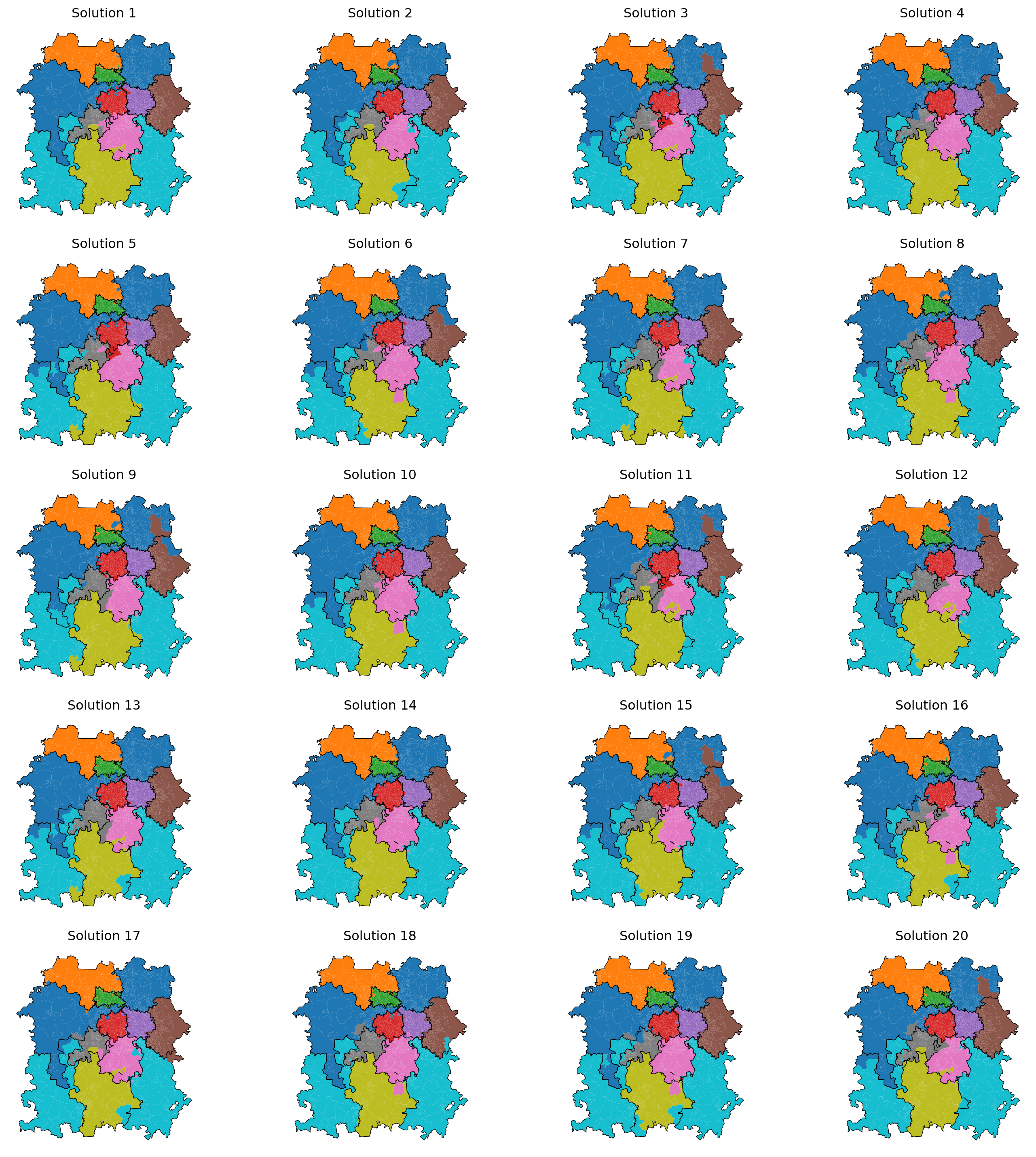

Warning

Many of thse solutions may perform better against the demand balancing criteria, but suffer from being shapes that are suboptimal in the real world.

We will explore how we may tackle that in future sections. We may choose to prioritise solutions that perform well on measures of compactness, for example. A wide range of compactness metrics exist, such as the Polsby-Popper score and the Reock score, among others.

Additional options are the indentation score (convex hull comparison) and the area to perimeter ratio to check for regions with long, thin corridors.

We can also look at measures of connectivity like the edge cut score, which looks at how many border connections would be required to cut off a region’s connectivity.

For example, the light blue region on the left here would require very little change to cut it off from itself.

This would be better.

As we bring in additional metrics like real-world travel times into our scoring in subsequent chapters, we may naturally begin to develop ‘better’ regions.

33.4.5 Evaluating the solutions against the demand

Let’s initially evaluate our evolved solutions based on our original single metric, which is how well each solution balances demand across the regions (minimizing the difference in demand per region, looking at historical demand data).

Click here to view our ‘evaluate_solution()’ function from the previous chapter

def evaluate_solution(gdf,
                      allocation_column='centre_dispatcher_NEW',
                      demand_column="demand"):
    grouped_by_dispatcher = gdf.groupby(allocation_column)[[demand_column]].sum()
    mean_demand = grouped_by_dispatcher['demand'].mean()

    grouped_by_dispatcher['difference_from_mean'] = (grouped_by_dispatcher['demand'] - mean_demand).astype('int')

    return abs(grouped_by_dispatcher['difference_from_mean']).mean().round(1)

def evaluate_solution_dict(solution_dict, gdf,
                            allocation_column='centre_dispatcher',
                            demand_column="demand", territory_unit_column="LSOA11CD"):

    owned_territory_df = pd.DataFrame(
            [(key, value) for key, values in solution_dict.items() for value in values],
            columns=[f"{allocation_column}_NEW", territory_unit_column])
    gdf = pd.merge(gdf, owned_territory_df, on=territory_unit_column, how="left")

    grouped_by_dispatcher = gdf.groupby(f"{allocation_column}_NEW")[[demand_column]].sum()
    mean_demand = grouped_by_dispatcher['demand'].mean()

    grouped_by_dispatcher['difference_from_mean'] = (grouped_by_dispatcher['demand'] - mean_demand).astype('int')

    return abs(grouped_by_dispatcher['difference_from_mean']).mean().round(1)

import copy

evaluations_evolved_solutions = []

for i, sol in enumerate(solution):
    allocation_evaluation = evaluate_solution(sol.merge(demand, on="LSOA11CD"), allocation_column="centre_dispatcher_evolved")

    evaluations_evolved_solutions.append({
        'solution': f"e{i+1}",
        # We can't just pass the dictionary here due to the way python handles dictionaries
        # We need to explicitly take a copy of the dictionary
        'allocations': copy.deepcopy(sol.groupby('centre_dispatcher_evolved')['LSOA11CD'].apply(list).to_dict()),
        'result': allocation_evaluation
    })

evolution_solution_df = pd.DataFrame(evaluations_evolved_solutions)
evolution_solution_df['rank'] = evolution_solution_df['result'].rank(method='max')

evolution_solution_df.sort_values('rank')

	solution	allocations	result	rank
12	e13	{'Centre 1-1': ['E01009742', 'E01009745', 'E01...	9273.6	1.0
15	e16	{'Centre 1-1': ['E01009742', 'E01009745', 'E01...	9343.4	2.0
14	e15	{'Centre 1-1': ['E01009742', 'E01009745', 'E01...	9452.1	3.0
29	e30	{'Centre 1-1': ['E01009742', 'E01009745', 'E01...	9469.6	4.0
27	e28	{'Centre 1-1': ['E01009742', 'E01009745', 'E01...	9479.9	5.0
0	e1	{'Centre 1-1': ['E01009742', 'E01009745', 'E01...	9499.9	6.0
2	e3	{'Centre 1-1': ['E01009742', 'E01009745', 'E01...	9526.9	7.0
23	e24	{'Centre 1-1': ['E01009742', 'E01009745', 'E01...	9531.9	8.0
4	e5	{'Centre 1-1': ['E01009742', 'E01009745', 'E01...	9536.8	9.0
19	e20	{'Centre 1-1': ['E01009742', 'E01009745', 'E01...	9563.1	10.0
20	e21	{'Centre 1-1': ['E01009742', 'E01009745', 'E01...	9566.4	11.0
28	e29	{'Centre 1-1': ['E01009742', 'E01009745', 'E01...	9568.4	12.0
13	e14	{'Centre 1-1': ['E01009742', 'E01009745', 'E01...	9574.4	13.0
6	e7	{'Centre 1-1': ['E01009742', 'E01009745', 'E01...	9603.9	14.0
9	e10	{'Centre 1-1': ['E01009742', 'E01009745', 'E01...	9632.8	15.0
17	e18	{'Centre 1-1': ['E01009742', 'E01009745', 'E01...	9665.6	16.0
21	e22	{'Centre 1-1': ['E01009742', 'E01009745', 'E01...	9678.8	17.0
3	e4	{'Centre 1-1': ['E01009742', 'E01009745', 'E01...	9682.2	18.0
16	e17	{'Centre 1-1': ['E01009742', 'E01009745', 'E01...	9687.4	19.0
26	e27	{'Centre 1-1': ['E01009742', 'E01009745', 'E01...	9704.4	20.0
11	e12	{'Centre 1-1': ['E01009742', 'E01009745', 'E01...	9723.1	21.0
22	e23	{'Centre 1-1': ['E01009742', 'E01009745', 'E01...	9738.1	22.0
8	e9	{'Centre 1-1': ['E01009742', 'E01009745', 'E01...	9738.2	23.0
1	e2	{'Centre 1-1': ['E01009742', 'E01009745', 'E01...	9738.8	24.0
25	e26	{'Centre 1-1': ['E01009742', 'E01009745', 'E01...	9743.2	25.0
10	e11	{'Centre 1-1': ['E01009742', 'E01009745', 'E01...	9746.8	26.0
18	e19	{'Centre 1-1': ['E01009742', 'E01009745', 'E01...	9871.8	27.0
24	e25	{'Centre 1-1': ['E01009742', 'E01009745', 'E01...	9874.6	28.0
7	e8	{'Centre 1-1': ['E01009742', 'E01009745', 'E01...	9943.9	29.0
5	e6	{'Centre 1-1': ['E01009742', 'E01009745', 'E01...	10037.6	30.0

Let’s add the original random solutions into our ranking table.

initial_solution_df['what'] = 'random'
evolution_solution_df['what'] = 'evolved'

full_sol_df = pd.concat([initial_solution_df, evolution_solution_df])
full_sol_df['rank'] = full_sol_df['result'].rank(method='max')
full_sol_df.sort_values('rank')

	solution	allocations	result	rank	what
12	e13	{'Centre 1-1': ['E01009742', 'E01009745', 'E01...	9273.6	1.0	evolved
15	e16	{'Centre 1-1': ['E01009742', 'E01009745', 'E01...	9343.4	2.0	evolved
14	e15	{'Centre 1-1': ['E01009742', 'E01009745', 'E01...	9452.1	3.0	evolved
29	e30	{'Centre 1-1': ['E01009742', 'E01009745', 'E01...	9469.6	4.0	evolved
27	e28	{'Centre 1-1': ['E01009742', 'E01009745', 'E01...	9479.9	5.0	evolved
0	e1	{'Centre 1-1': ['E01009742', 'E01009745', 'E01...	9499.9	6.0	evolved
2	e3	{'Centre 1-1': ['E01009742', 'E01009745', 'E01...	9526.9	7.0	evolved
23	e24	{'Centre 1-1': ['E01009742', 'E01009745', 'E01...	9531.9	8.0	evolved
4	e5	{'Centre 1-1': ['E01009742', 'E01009745', 'E01...	9536.8	9.0	evolved
19	e20	{'Centre 1-1': ['E01009742', 'E01009745', 'E01...	9563.1	10.0	evolved
20	e21	{'Centre 1-1': ['E01009742', 'E01009745', 'E01...	9566.4	11.0	evolved
28	e29	{'Centre 1-1': ['E01009742', 'E01009745', 'E01...	9568.4	12.0	evolved
13	e14	{'Centre 1-1': ['E01009742', 'E01009745', 'E01...	9574.4	13.0	evolved
6	e7	{'Centre 1-1': ['E01009742', 'E01009745', 'E01...	9603.9	14.0	evolved
9	e10	{'Centre 1-1': ['E01009742', 'E01009745', 'E01...	9632.8	15.0	evolved
9	10	{'Centre 2-5': ['E01031187', 'E01031195', 'E01...	9651.1	16.0	random
17	e18	{'Centre 1-1': ['E01009742', 'E01009745', 'E01...	9665.6	17.0	evolved
21	e22	{'Centre 1-1': ['E01009742', 'E01009745', 'E01...	9678.8	18.0	evolved
3	e4	{'Centre 1-1': ['E01009742', 'E01009745', 'E01...	9682.2	19.0	evolved
16	e17	{'Centre 1-1': ['E01009742', 'E01009745', 'E01...	9687.4	20.0	evolved
26	e27	{'Centre 1-1': ['E01009742', 'E01009745', 'E01...	9704.4	21.0	evolved
11	e12	{'Centre 1-1': ['E01009742', 'E01009745', 'E01...	9723.1	22.0	evolved
22	e23	{'Centre 1-1': ['E01009742', 'E01009745', 'E01...	9738.1	23.0	evolved
8	e9	{'Centre 1-1': ['E01009742', 'E01009745', 'E01...	9738.2	24.0	evolved
1	e2	{'Centre 1-1': ['E01009742', 'E01009745', 'E01...	9738.8	25.0	evolved
25	e26	{'Centre 1-1': ['E01009742', 'E01009745', 'E01...	9743.2	26.0	evolved
10	e11	{'Centre 1-1': ['E01009742', 'E01009745', 'E01...	9746.8	27.0	evolved
5	6	{'Centre 2-5': ['E01031187', 'E01031218', 'E01...	9842.8	28.0	random
18	e19	{'Centre 1-1': ['E01009742', 'E01009745', 'E01...	9871.8	29.0	evolved
24	e25	{'Centre 1-1': ['E01009742', 'E01009745', 'E01...	9874.6	30.0	evolved
7	e8	{'Centre 1-1': ['E01009742', 'E01009745', 'E01...	9943.9	31.0	evolved
5	e6	{'Centre 1-1': ['E01009742', 'E01009745', 'E01...	10037.6	32.0	evolved
14	15	{'Centre 2-5': ['E01031187', 'E01031208', 'E01...	10811.3	33.0	random
6	7	{'Centre 2-5': ['E01031187', 'E01031218', 'E01...	10869.2	34.0	random
10	11	{'Centre 2-5': ['E01031187', 'E01031204', 'E01...	11043.4	35.0	random
8	9	{'Centre 2-5': ['E01031187', 'E01031208', 'E01...	11218.6	36.0	random
17	18	{'Centre 2-5': ['E01031187', 'E01031195', 'E01...	11401.2	37.0	random
7	8	{'Centre 2-5': ['E01031187', 'E01031218', 'E01...	12088.3	38.0	random
1	2	{'Centre 2-5': ['E01031187', 'E01031204', 'E01...	12226.2	39.0	random
4	5	{'Centre 2-5': ['E01031187', 'E01031204', 'E01...	12399.0	40.0	random
2	3	{'Centre 2-5': ['E01031187', 'E01031195', 'E01...	12418.8	41.0	random
3	4	{'Centre 2-5': ['E01031187', 'E01031188', 'E01...	12567.1	42.0	random
15	16	{'Centre 2-5': ['E01031187', 'E01031188', 'E01...	12831.8	43.0	random
16	17	{'Centre 2-5': ['E01031187', 'E01031208', 'E01...	13103.8	44.0	random
19	20	{'Centre 2-5': ['E01031187', 'E01031195', 'E01...	13126.5	45.0	random
18	19	{'Centre 2-5': ['E01031187', 'E01031213', 'E01...	13196.2	46.0	random
13	14	{'Centre 2-5': ['E01031187', 'E01031218', 'E01...	13443.9	47.0	random
11	12	{'Centre 2-5': ['E01031187', 'E01031188', 'E01...	13632.6	48.0	random
12	13	{'Centre 2-5': ['E01031187', 'E01031204', 'E01...	13954.4	49.0	random
0	1	{'Centre 2-5': ['E01031187', 'E01031204', 'E01...	14735.8	50.0	random

import plotly.express as px

# Sort by 'result' to ensure correct order
full_sol_df = full_sol_df.sort_values("result", ascending=True)

# Convert 'solution' to a string (if it's not already)
full_sol_df["solution"] = full_sol_df["solution"].astype(str)

# Create the plot and enforce sorted order
fig = px.bar(
    full_sol_df,
    x="solution",
    y="result",
    color="what",
    category_orders={"solution": full_sol_df["solution"].tolist()}  # Enforce order
)

fig.show()

We will now take a specified portion of these solutions, evolve them, evaluate them again, and continue.

We will also start tracking how good the best solution we are achieving is after each evolution.

We will repeat this 1000 times, plotting the value for our best solution over time to see how much better we can make the solution with sufficient permutations.

Tip

Coming soon!

Let’s plot what we started with versus our best 10 solutions at the end of the process.

Here is our final start-to-finish code for generating and evaluating the solutions.

Tip

Coming soon!

---

1. Meskarian R, Penn ML, Williams S, Monks T (2017) A facility location model for analysis of current and future demand for sexual health services. PLoS ONE 12(8): e0183942. https://doi.org/10.1371/journal.pone.0183942

2. A genetic algorithm for calculating minimum distance between convex and concave bodies - Scientific Figure on ResearchGate. Available from: https://www.researchgate.net/figure/Local-versus-global-optimum_fig1_228563694 [accessed 9 Apr, 2024]