32Boundary Problems - Creating and Evaluating Simple Solutions
32.1 Generating and representing new boundaries
When we come to modifying our existing boundaries, we are going to generate a large set of random new boundaries and test them.
Note
Remember - in our problem statement, we specified that boundaries in our problem cannot cross through the middle of an LSOA. You would need to apply a different approach if this is not true in your case.
Tip
If you have a series of pre-selected solutions to try, the code in the following sections can be adapted to use those solutions rather than the randomly-generated solutions.
First, we will define the LSOAs that each LSOA has a continuous boundary with. These will form part of a possible series of solutions. To do this, we’ll be using the .touches method in geopandas.
In this case, a solution must meet a criteria
every polygon must be assigned to a dispatcher
no polygon can be assigned to more than one dispatcher
dispatcher boundaries must be continuous; regions belonging to a dispatcher cannot be entirely separated from the rest of their dispatch area
At this point, we are not trying to do anything to balance our objectives like equalising the number of calls they are going to; instead, we are simply coming up with possibilities. We’ll actually test them out in the next chapter.
32.1.1 The Process
To create a solution that scales well to any number of dispatchers, we will have the dispatchers start with a single randomly-selected patch from their existing location (though we will also code in an option to always start from a single specified point).
Then, on each ‘turn’, they will randomly choose another patch from the patches that share a boundary with the first patch. There is a small (adjustable) possibility on each turn that they will not opt to take a turn; this will be part of our strategy to ensure that not every dispatcher ends up with solutions containing exactly the same number of regions.
On each subsequent turn, they will randomly select another region that touches any part of their existing region. If the region that is selected is a region that they already have in their ‘patch’, or a region that is already ‘owned’ by another ‘player’, then their ‘go’ ends without them gaining any additional territory. However, if they have randomly selected an ‘unowned’ spot, this is then added to their
Here’s an example of one of our ‘walks’ building up. This only shows the first few steps, but eventually it would continue until the whole patch was covered, following the same pattern.
Here, player 1’s patches are red, and player 2’s are purple. Light blue patches are those not yet owned by either player.
This just showed us building up two patches, but more patches could be built with a larger number of ‘players’, with a third player being represented in yellow here.
Tip
Remember - due to the randomness we will introduce in multiple ways, each generated solution will be slightly different.
Tip
Again, this is not the only way we can start to generate solutions here!
This is one of many approaches you could take.
Note
When we come to apply a evolutionary or genetic algorithm approach to this problem in a later chapter, we will need to change how we represent our solutions; for now, however, we can just put together lists of LSOAs that will belong to each dispatcher.
Let’s write and apply this function to generate a series of randomly generated solutions for our problem, which we will subsequently move on to evaluating.
32.1.2 Our starting dataframe
To start with, let’s load our boundary data back in. Head back to the previous chapter if any of this feels unfamiliar!
/home/sammi/.local/lib/python3.10/site-packages/geopandas/geodataframe.py:1528: SettingWithCopyWarning:


A value is trying to be set on a copy of a slice from a DataFrame.
Try using .loc[row_indexer,col_indexer] = value instead

See the caveats in the documentation: https://pandas.pydata.org/pandas-docs/stable/user_guide/indexing.html#returning-a-view-versus-a-copy
32.1.3 Getting the Neighbours
Before we start worrying about the allocations, we first want to generate a column that contains a list of all of the neighbours of a given cell. This will be a lot more efficient than trying to calculate the neighbours from scratch each time we want to pick a new one - and it’s not like the neighbours will change.
GenAI Alert - This code was modified from a suggested approach provided by ChatGPT
def add_neighbors_column(gdf):""" Adds a column to the GeoDataFrame containing lists of indices of neighboring polygons based on the 'touches' method. """ gdf = gdf.copy() neighbors = []for idx, geom in gdf.geometry.items(): touching = gdf[gdf.geometry.touches(geom)]["LSOA11CD"].tolist() neighbors.append(touching) gdf["neighbors"] = neighborsreturn gdfbham_region = add_neighbors_column(bham_region)bham_region[['LSOA11CD', 'LSOA11NM', 'LSOA11NMW', 'geometry', 'neighbors']].head()
32.1.4 Making a dictionary of the existing allocations
First, let’s make ourselves a dictionary. In this dictionary, the keys will be the centre/dispatcher, and the values will be a list of all LSOAs that currently belong to that dispatcher.
# Get a list of the unique dispatchersdispatchers = bham_region['centre_dispatcher'].unique()dispatchers.sort()dispatcher_starting_allocation_dict = {}for dispatcher in dispatchers: dispatcher_allocation = bham_region[bham_region["centre_dispatcher"] == dispatcher] dispatcher_starting_allocation_dict[dispatcher] = dispatcher_allocation["LSOA11CD"].unique()
Let’s look at what that looks like for one of the dispatchers. Using this, we can access a full list of their LSOAs whenever we need it.
To start with, let’s build up our random walk algorithm step-by-step. At the end of this section, we’ll turn it into a reusable functions with some parameters to make it easier to use. After that, we’ll work on building a reusable function to help us quickly evaluate each solution we generate.
32.1.5 Generating starting allocations
The first step will be to generate an initial starting point for each dispatcher.
There are a couple of different approaches we could take here - and maybe we’ll give our eventual algorithm the option to pick from several options.
Option 1 - Use our new dictionary to select a random starting LSOA for each of our dispatchers from within their existing territories.
Option 2 - Start with the most central region of the existing regions for each dispatcher.
Option 3 - Provide each dispatcher with an entirely random starting point, regardless of the historical boundaries.
Option 1
We could use our new dictionary to select a random starting LSOA for each of our dispatchers from within their existing territories. This will give us plenty of randomness - but we may find ourselves with walks that start very near the edge of our original patch, giving us very different boundaries to what existed before.
import randomrandom_solution_starting_dict = {}for key, value in dispatcher_starting_allocation_dict.items(): random_solution_starting_dict[key] = random.choice(value)random_solution_starting_dict
We’ll also be using a dataframe from the previous chapter - the code for this can be found in the expander if you want to revisit this.
Click here to see the code for generating our dispatch boundaries dataframe
# Group by the specified columngrouped_dispatcher_gdf = bham_region.groupby("centre_dispatcher")# Create a new GeoDataFrame for the boundaries of each groupboundary_list = []for group_name, group in grouped_dispatcher_gdf:# Combine the polygons in each group into one geometry combined_geometry = group.unary_union# Get the boundary of the combined geometry boundary = combined_geometry.boundary# Add the boundary geometry and the group name to the list boundary_list.append({'group': group_name, 'boundary': boundary})# Create a GeoDataFrame from the list of boundariesgrouped_dispatcher_gdf_boundary = geopandas.GeoDataFrame(boundary_list, geometry='boundary', crs=bham_region.crs)grouped_dispatcher_gdf_boundary.head()
group
boundary
0
Centre 1-1
MULTILINESTRING ((368935.969 274516.594, 36824...
1
Centre 1-2
LINESTRING (412258.535 300984.197, 411756.668 ...
2
Centre 1-3
LINESTRING (381775.908 282326.500, 380577.001 ...
3
Centre 1-4
LINESTRING (388885.341 295185.385, 388630.406 ...
4
Centre 1-5
LINESTRING (388258.095 285110.427, 388666.258 ...
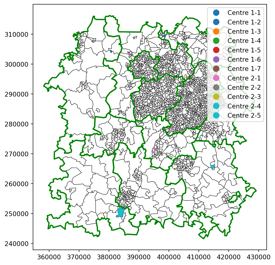
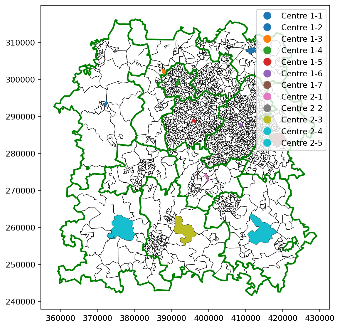
Some of the regions are quite small, so it may be hard to see them all!
# First, let's plot the outline of our entire regionax = bham_region.plot( figsize=(10,7), edgecolor='black', linewidth=0.5, color="white" )# Let's use our new function to generate a series of random starting patchessol = create_random_starting_dict(dispatcher_starting_allocation_dict)# We can filter our existing dataframe of allocations to just the starting patchesrandom_solution_start = bham_region[bham_region['LSOA11CD'].isin(sol.values())]# Finally, we plot those on the same plot, colouring by centre-dispatcher comborandom_solution_start.plot( ax=ax, column="centre_dispatcher", legend=True)# Let's also visualise the historical boundariesgrouped_dispatcher_gdf_boundary.plot( ax=ax, linewidth=2, edgecolor="green")
Option 2
Another alternative is to start with the most central region of the existing regions for each dispatcher.
from shapely.geometry import Pointdef find_most_central_polygon(gdf):""" Finds the most central polygon in a GeoDataFrame based on centroid proximity to the mean centroid. """# Compute centroids of individual polygons gdf["centroid"] = gdf.geometry.centroid# Calculate the mean centroid (central point) mean_centroid = gdf.geometry.unary_union.centroid# Compute distances from each centroid to the mean centroid gdf["distance_to_mean"] = gdf["centroid"].distance(mean_centroid)# Find the polygon with the minimum distance central_polygon = gdf.loc[gdf["distance_to_mean"].idxmin()]return central_polygondef get_central_polygon_per_group(gdf, grouping_col):return gdf.groupby(grouping_col, group_keys=False).apply(find_most_central_polygon).drop(columns=["centroid", "distance_to_mean"])most_central = get_central_polygon_per_group(bham_region, "centre_dispatcher")most_central
FID
LSOA11CD
LSOA11NM
LSOA11NMW
BNG_E
BNG_N
LONG
LAT
GlobalID
geometry
region
neighbors
Region
Centre
Dispatcher
centre_dispatcher
centre_dispatcher
Centre 1-1
28095
E01028832
Shropshire 033A
Shropshire 033A
372082
293080
-2.41300
52.53487
945b5cd8-45bd-4f3a-8834-88082caa2473
POLYGON ((372799.246 293568.354, 372202.351 29...
Shropshire
[E01028828, E01028830, E01028833, E01028834, E...
Shropshire
Centre 1
1
Centre 1-1
Centre 1-2
28764
E01029518
Lichfield 007D
Lichfield 007D
411232
307750
-1.83534
52.66736
421455c3-c4b7-4505-880d-8412aa14c957
POLYGON ((412402.657 308666.999, 412311.329 30...
Lichfield
[E01029488, E01029512, E01029519, E01029520, E...
Lichfield
Centre 1
2
Centre 1-2
Centre 1-3
28875
E01029631
South Staffordshire 009E
South Staffordshire 009E
388142
301842
-2.17656
52.61423
6d0e4c4c-bf69-4f68-a086-46d1a80854d9
POLYGON ((387776.111 302749.666, 388831.796 30...
South Staffordshire
[E01010544, E01010546, E01029613, E01029615, E...
South Staffordshire
Centre 1
3
Centre 1-3
Centre 1-4
10215
E01010521
Wolverhampton 020F
Wolverhampton 020F
391688
299252
-2.12412
52.59101
5966f7f1-af15-4226-9d1e-6316101606b5
POLYGON ((391805.204 300349.956, 392207.285 29...
Wolverhampton
[E01010426, E01010443, E01010463, E01010464, E...
Wolverhampton
Centre 1
4
Centre 1-4
Centre 1-5
9743
E01010043
Sandwell 025B
Sandwell 025B
395995
288750
-2.06041
52.49665
3be670e2-fde7-4251-ad24-56335b4c30df
POLYGON ((396648.514 288801.684, 396670.147 28...
Sandwell
[E01009843, E01009871, E01009888, E01009890, E...
Sandwell
Centre 1
5
Centre 1-5
Centre 1-6
8940
E01009204
Birmingham 052E
Birmingham 052E
408607
287498
-1.87467
52.48535
e1aaf4f1-f7a4-4e98-9d74-855033a27584
POLYGON ((409131.178 287204.736, 408353.160 28...
Birmingham
[E01009199, E01009201, E01009203, E01033561, E...
Birmingham
Centre 1
6
Centre 1-6
Centre 1-7
9809
E01010109
Solihull 009A
Solihull 009A
418665
283710
-1.72677
52.45104
d03080c8-368a-46af-9fed-b27cc051518e
POLYGON ((419807.904 285425.582, 419899.498 28...
Solihull
[E01009318, E01009320, E01010108, E01010110, E...
Solihull
Centre 1
7
Centre 1-7
Centre 2-1
31345
E01032149
Bromsgrove 006D
Bromsgrove 006D
399455
274007
-2.00941
52.36413
3b13e41d-e470-47c0-9830-cd654e36a32e
POLYGON ((399816.607 273656.656, 400092.197 27...
Bromsgrove
[E01032143, E01032144, E01032148, E01032150, E...
Bromsgrove
Centre 2
1
Centre 2-1
Centre 2-2
31667
E01032477
Wyre Forest 008D
Wyre Forest 008D
381330
275610
-2.27568
52.37821
4f0cf516-7c4b-4b61-a4da-da4423304f43
POLYGON ((381780.507 275809.361, 381793.089 27...
Wyre Forest
[E01032451, E01032470, E01032471, E01032476, E...
Wyre Forest
Centre 2
2
Centre 2-2
Centre 2-3
31535
E01032345
Wychavon 007A
Wychavon 007A
393387
259105
-2.09823
52.23011
b7f03ca0-aac0-4e29-b86c-95dd4a796fce
POLYGON ((396864.091 258452.893, 396188.712 25...
Wychavon
[E01032346, E01032360, E01032361, E01032362, E...
Wychavon
Centre 2
3
Centre 2-3
Centre 2-4
31391
E01032199
Malvern Hills 002C
Malvern Hills 002C
376434
260160
-2.34652
52.23913
c4525de8-e8d8-4d8b-9610-d887d58dbabb
POLYGON ((378353.003 262294.903, 378414.904 26...
Malvern Hills
[E01014001, E01032179, E01032181, E01032182, E...
Malvern Hills
Centre 2
4
Centre 2-4
Centre 2-5
30398
E01031187
Stratford-on-Avon 007A
Stratford-on-Avon 007A
414464
258742
-1.78965
52.22670
679c1798-8095-4712-a9b9-c495cca9dadd
POLYGON ((416799.690 260453.800, 416633.500 25...
Stratford-on-Avon
[E01031188, E01031195, E01031204, E01031208, E...
Stratford-on-Avon
Centre 2
5
Centre 2-5
Let’s plot this.
# First, let's plot the outline of our entire regionax = bham_region.plot( figsize=(10,7), edgecolor='black', linewidth=0.5, color="white" )# Plot those on the same plot, colouring by centre-dispatcher combomost_central.plot( ax=ax, column="centre_dispatcher", legend=True)# Let's also visualise the historical boundariesgrouped_dispatcher_gdf_boundary.plot( ax=ax, linewidth=2, edgecolor="green")
You can see that in some regions the most central point can still be on a boundary, even
32.1.6 Generating our new regions
As a recap, what we want to do now is introduce a number of ‘players’ who will play a territory-grabbing game. Our ‘players’ - the dispatchers - will each have a single turn, pass control to the next dispatcher, and so on.
On each turn, they will be presented with a long list of the regions that share a boundary with any of their existing territories. They will then choose a territory at random from that list.
However, this doesn’t mean their territory will expand on every turn.
The territory that they choose could be one of their existing territories (as we are checking for a boundary with any of their existing territories on a per-territory basis - not the outer boundary of their entire territory)
There will also be a random chance introduced that they just don’t take a go
They may also try to take a territory that is already owned by a different dispatcher, in which case they will not gain anything on the turn - though we could always add in an option like them ‘battling’ for the territory
So let’s start coding this!
First, let’s work on the logic for selecting a territory from their existing list. We’ll just do this with a single dispatcher for now.
We’ll filter down to this and remind ourselves what the available data on neighbouring territory looks like.
# We'll start with dispatcher 5 from centre 2, and we'll use the most central point of their existing territorydispatcher ="Centre 2-5"starting_point = most_central[most_central["centre_dispatcher"] == dispatcher]starting_point['neighbors']
Let’s now pick a random neighbour, and work out a way to store the new allocations so we can ensure we know who owns what territory, and we don’t end up with a situation where two dispatchers own the same territory.
Fantastic! We now have a simple way to get and store this.
Let’s have a go at giving another dispatcher a turn to grab territory.
dispatcher ="Centre 1-1"starting_point = most_central[most_central["centre_dispatcher"] == dispatcher]# This time we add to the existing dict rather than setting it up anewowned_territory_dict[dispatcher] = [starting_point['LSOA11CD'].values[0]]# Now we do our random selectionselected_territory = random.choice(starting_point['neighbors'].values[0])owned_territory_dict[dispatcher].append(selected_territory)owned_territory_dict
This is a good step, and for now we’re unlikely to run into the issue of different dispatchers owning the same territory - though it’s not impossible! So let’s add in another dispatcher, but this time we’ll check first that it’s not owned by anyone.
First, let’s pull back the full list of owned territories from our dict.
We’ll need to convert this into a single list. We could use a for loop, or a list comprehension.
territory_list = [element for sub_list inlist(owned_territory_dict.values()) for element in sub_list]# By using set, then list on the result of that, we get a list of unique valuesterritory_list =list(set(territory_list))territory_list
dispatcher ="Centre 1-5"starting_point = most_central[most_central["centre_dispatcher"] == dispatcher]owned_territory_dict[dispatcher] = [starting_point['LSOA11CD'].values[0]]selected_territory = random.choice(starting_point['neighbors'].values[0])# Only add the territory if it's not already in the list of owned territoryif selected_territory notin territory_list: owned_territory_dict[dispatcher].append(selected_territory)owned_territory_dict
That’s most of the key elements of our function written now - so let’s actually turn it into a function that will continue to run until all of the territory has been allocated.
For clarity and ease of use, we’ll set up our defaults to relate to our current objects - but for a more reusable function, it may be better to avoid defaults but be very clear in the docstring what is expected as an input, and add in some error handling to manage cases that don’t match.
def generate_random_territory_allocation( gdf=bham_region, territory_unit_column="LSOA11CD", player_list=bham_region["centre_dispatcher"].unique(), player_column="centre_dispatcher", starting_territories=most_central, neighbor_column='neighbors', skipgo_chance=0.03, return_df=True ):# Initialise the territory list as the starting territories owned_territory_list =list(starting_territories[territory_unit_column].unique())# Set up the starting territory for each individual and have each player have their first gofor player in player_list: starting_point = starting_territories[starting_territories[player_column] == player] owned_territory_dict[player] = [starting_point[territory_unit_column].values[0]] selected_territory = random.choice(starting_point['neighbors'].values[0])# Only add the territory if it's not already in the list of owned territoryif selected_territory notin owned_territory_list: owned_territory_dict[player].append(selected_territory)# As we're now going to be iterating and checking throughout, we can just# maintain the owned territory list as we go along, which is a bit easier and# more efficient than generating it from the territory dict each time owned_territory_list.append(selected_territory)# Keep going through the following process until all territory has been allocatedwhilelen(owned_territory_list) <len(gdf[territory_unit_column].unique()):# Go around all individualsfor player in player_list:if random.random() > skipgo_chance:# Select a random existing territory from the list of owned territories chosen_owned_territory = random.choice(owned_territory_dict[player])# Then find the neighbours neighbors = gdf[gdf[territory_unit_column] == chosen_owned_territory][neighbor_column].values[0]# Choose a random neighbour and update the list of owned territories... selected_territory = random.choice(neighbors)#... if not already ownedif selected_territory notin owned_territory_list: owned_territory_dict[player].append(selected_territory) owned_territory_list.append(selected_territory)if return_df: owned_territory_df = pd.DataFrame( [(key, value) for key, values in owned_territory_dict.items() for value in values], columns=[f"{player_column}_NEW", territory_unit_column])return pd.merge(gdf, owned_territory_df, on=territory_unit_column, how="left")else:return owned_territory_dict
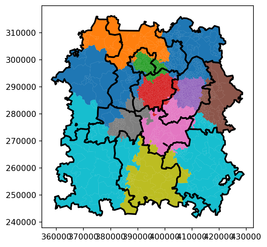
Let’s try our new function out and see what it returns.
Let’s see how much this differs from the original allocation.
# Plot the new boundaries using coloursax = random_allocation_test.plot( column="centre_dispatcher_NEW")# Visualise the historical boundariesgrouped_dispatcher_gdf_boundary.plot( ax=ax, linewidth=2, edgecolor="black")
32.1.8 Comparing a new solution to the current allocation
For now, we’re going to judge a solution on a single criteria - the average absolute difference in demand across
This is calculated by calculating the difference in total demand experiences by one dispatcher from the average across all dispatchers. We then take the absolute value - i.e. if the difference is negative (the dispatcher received fewer calls than the average), we will turn it into a postive. Finally, we take the average across these values.
And now let’s try this out on our original and new solutions
demand = pd.read_csv("demand_pop_bham.csv")random_allocation_test = random_allocation_test.merge(demand, on="LSOA11CD")original_result = evaluate_solution(random_allocation_test, allocation_column='centre_dispatcher')new_result = evaluate_solution(random_allocation_test, allocation_column='centre_dispatcher_NEW')print(f"Original Allocation: {original_result}")print(f"Random Solution 1: {new_result}")if original_result > new_result:print("The randomly generated solution gives a more even allocation of events than the original dispatcher allocations")else:print("The randomly generated solution is worse than the original dispatcher allocations")
Original Allocation: 20934.4
Random Solution 1: 13014.4
The randomly generated solution gives a more even allocation of events than the original dispatcher allocations
32.2 Trying this out for more solutions
Let’s now run this for 20 different solutions and store the results.
def evaluate_solution_dict(solution_dict, gdf, allocation_column='centre_dispatcher', demand_column="demand", territory_unit_column="LSOA11CD"): owned_territory_df = pd.DataFrame( [(key, value) for key, values in solution_dict.items() for value in values], columns=[f"{allocation_column}_NEW", territory_unit_column]) gdf = pd.merge(gdf, owned_territory_df, on=territory_unit_column, how="left") grouped_by_dispatcher = gdf.groupby(f"{allocation_column}_NEW")[[demand_column]].sum() mean_demand = grouped_by_dispatcher['demand'].mean() grouped_by_dispatcher['difference_from_mean'] = (grouped_by_dispatcher['demand'] - mean_demand).astype('int')returnabs(grouped_by_dispatcher['difference_from_mean']).mean().round(1)
# Ensure our dataframe has the demand columnimport copybham_region = bham_region.merge(demand, on="LSOA11CD")solutions = []for i inrange(20): allocations = generate_random_territory_allocation(return_df=False) allocation_evaluation = evaluate_solution_dict(solution_dict=allocations, gdf=bham_region) solutions.append({'solution': i+1,# We can't just pass the dictionary here due to the way python handles dictionaries# We need to explicitly take a copy of the dictionary'allocations': copy.deepcopy(allocations),'result': allocation_evaluation })solution_df = pd.DataFrame(solutions)solution_df['rank'] = solution_df['result'].rank(method='max')solution_df.to_pickle('solutions_example.pkl')solution_df.sort_values('rank', ascending=True)